Algorithm Basics and Complexity Analysis

From containers to algorithms

In Introduction to Data Structures, you practiced thinking about data by its shape and operations: access, search, insert, delete, update, and iterate.

Now we add the next layer:

How does the work grow as the input grows?

That question is the heart of algorithm analysis. It lets you compare solutions before you submit code, and it helps you choose between approaches when both seem to work on small examples.

In a 30-day crash course, this skill is a multiplier: every problem you revisit later becomes easier to evaluate.

Complexity is about scaling

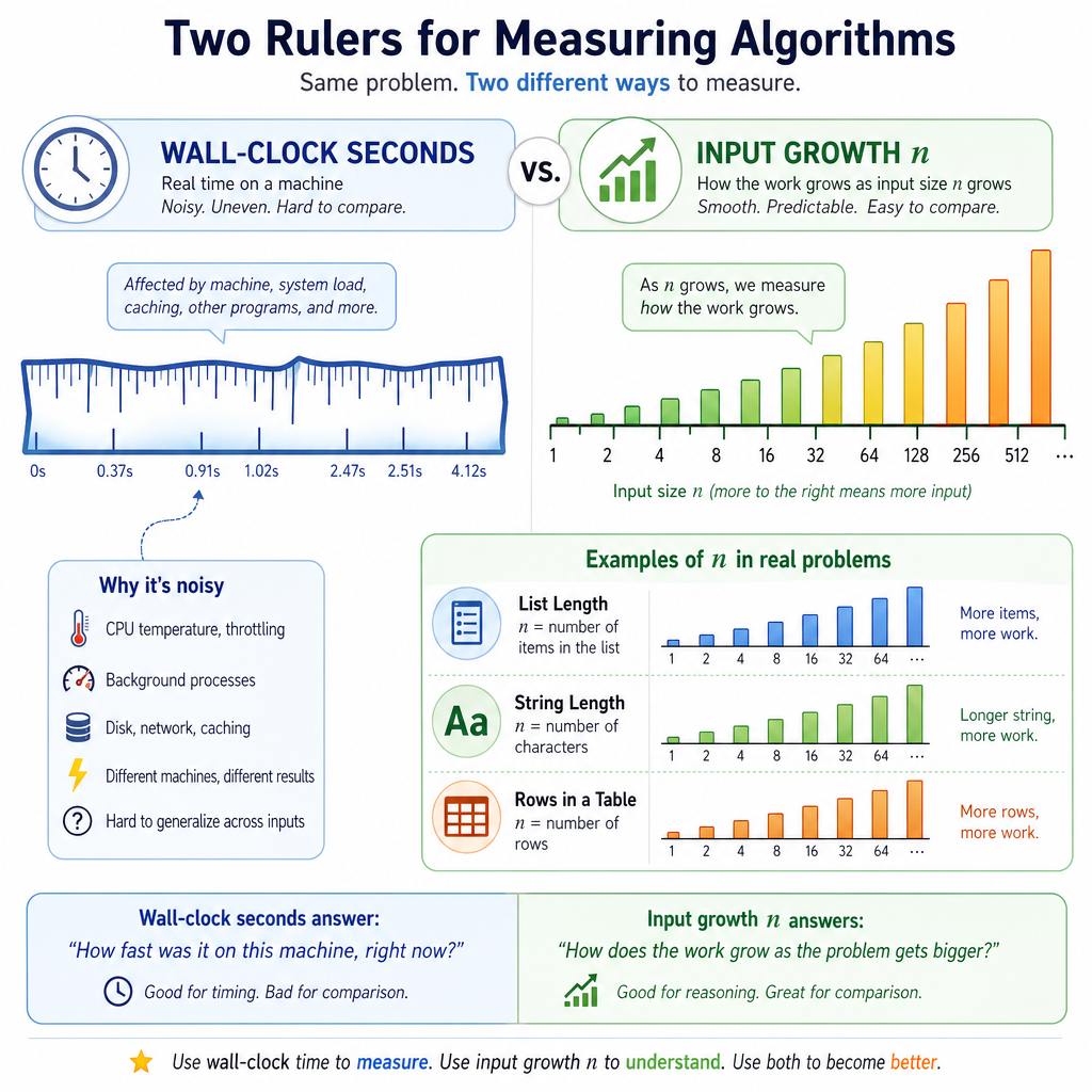
When analyzing an algorithm, we usually call the input size n.

Examples:

• A list with n numbers
• A string with n characters
• A table with n rows
• A collection of n users

We do not mainly ask, "How many seconds does this take on my laptop?"

Instead, we ask:

If n doubles, triples, or becomes huge, how does the amount of work change?

This is why complexity analysis is more stable than timing. Hardware, Python version, and background apps can affect seconds. Growth patterns tell you something deeper.

Count the repeated work

A beginner-friendly way to estimate runtime is to count how many times the core operation runs.

A single loop over n items grows linearly: O(n).

A loop inside another loop often grows quadratically: O(n²).

You do not need exact stopwatch numbers. You need the growth pattern.

```python
def count_operations(n):
    single_loop_steps = 0
    for i in range(n):
        single_loop_steps += 1

    nested_loop_steps = 0
    for i in range(n):
        for j in range(n):
            nested_loop_steps += 1

    return single_loop_steps, nested_loop_steps

for n in [5, 10, 20]:
    single, nested = count_operations(n)
    print(f"n={n}: single loop={single}, nested loop={nested}")
```

A function loops through a list of length n once and does constant-time work for each item.

What is the most appropriate Big O runtime?

The vocabulary of growth

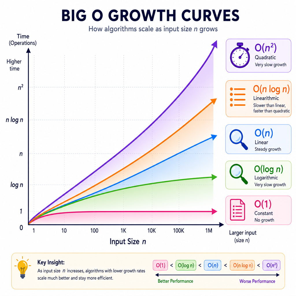
Big O describes the dominant growth trend as input gets large.

Common shapes:

• O(1): constant time
• O(log n): grows very slowly, often from repeatedly cutting the search space
• O(n): one pass through the input
• O(n log n): common in efficient sorting
• O(n²): comparing many pairs or using nested loops over the same input

Tiny mental graph:

work
 ^
 |                 O(n²)
 |             /
 |         O(n log n)
 |       /
 |    O(n)
 |  O(log n)
 |__O(1)________________> n

Do not memorize this as trivia. Use it to predict which solution will survive larger test cases.

True or false:

If an algorithm does one loop over n items, then another separate loop over the same n items, its runtime is usually simplified to O(n).

Same goal, different growth

Searching is a great place to see complexity in action.

If data is unsorted, you may need to check items one by one: O(n).

If data is sorted, you can sometimes repeatedly cut the search range in half: O(log n).

The important habit is not just naming the runtime. Ask what condition makes the faster method possible.

```python
def linear_search(nums, target):
    steps = 0
    for index, value in enumerate(nums):
        steps += 1
        if value == target:
            return index, steps
    return -1, steps


def binary_search(nums, target):
    left, right = 0, len(nums) - 1
    steps = 0

    while left <= right:
        steps += 1
        mid = (left + right) // 2
        if nums[mid] == target:
            return mid, steps
        elif nums[mid] < target:
            left = mid + 1
        else:
            right = mid - 1

    return -1, steps

nums = list(range(0, 64, 2))
target = 62

print("Linear search:", linear_search(nums, target))
print("Binary search:", binary_search(nums, target))
```

Simplify this Big O expression by keeping only the dominant term and dropping constants:

O(n² + 3n + 20) = ___

Fill in the blank: _____________

Runtime is not the only cost

Complexity analysis also includes space complexity: how much extra memory your algorithm uses as input grows.

Two solutions can both be O(n) time but use different amounts of extra memory.

Common examples:

• Building a new list of size n: O(n) extra space
• Keeping only a few counters or variables: O(1) extra space

In interviews and timed practice, say both when relevant: "This is O(n) time and O(1) extra space."

```python
def squares_copy(nums):
    result = []
    for num in nums:
        result.append(num * num)
    return result


def running_sum(nums):
    total = 0
    for num in nums:
        total += num
    return total

numbers = [1, 2, 3, 4, 5]

print("New list:", squares_copy(numbers))
print("Running sum:", running_sum(numbers))
print("Extra list length created by squares_copy:", len(squares_copy(numbers)))
```

Your analysis checklist

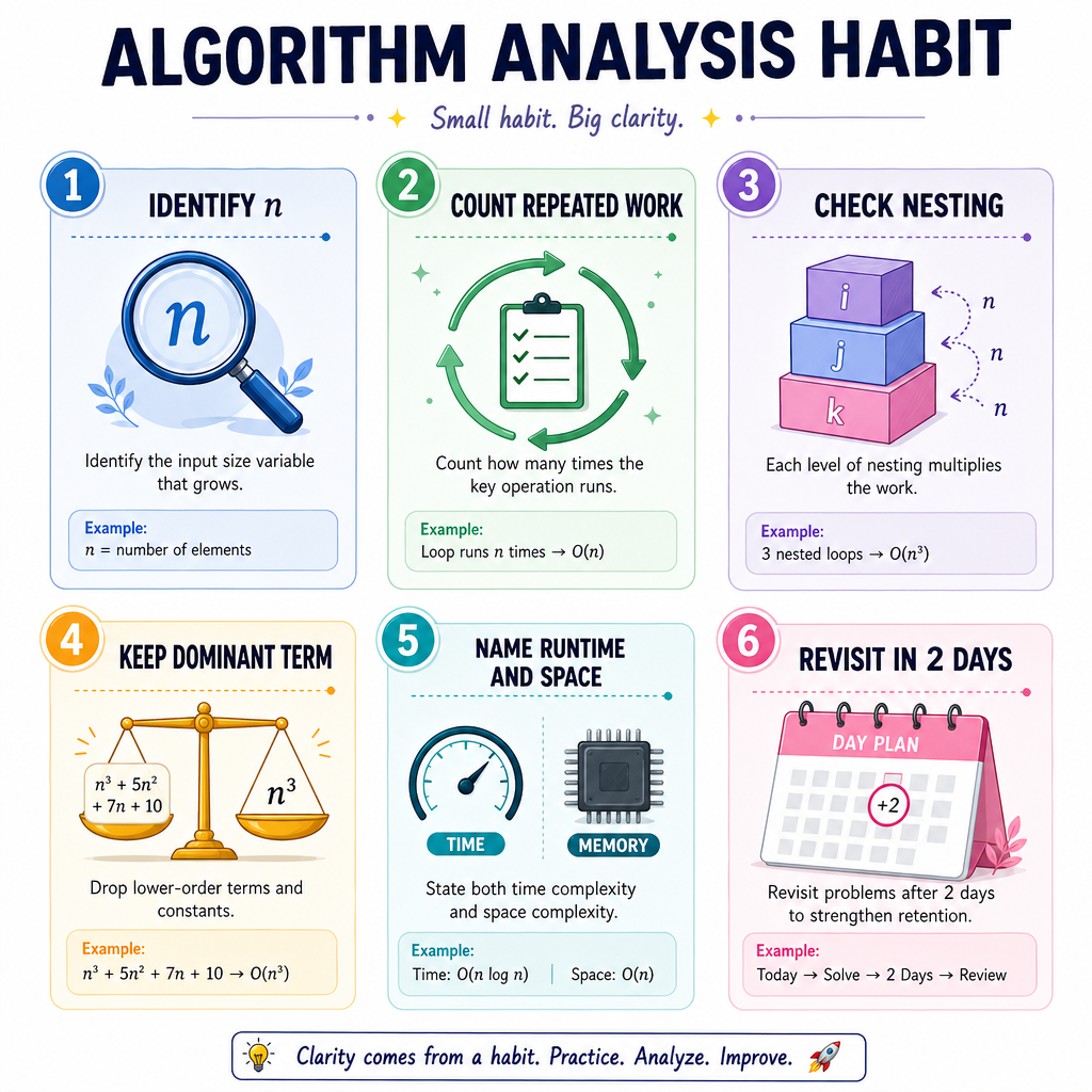
For every easy or medium problem this week, practice this quick routine:

1. Identify the input size: what is n?
2. Count the repeated work.
3. Look for nested repetition.
4. Keep the dominant term.
5. Name runtime and extra space.
6. Revisit the same problem in about 2 days and explain the complexity again.

This connects directly back to Introduction to Data Structures: first choose the structure that supports the operations, then analyze how the algorithm using it grows.

Next, we will use this same lens when functions call themselves in Recursive Algorithms and Backtracking.