Matplotlib
Let us first install the library matplotlib. We can do it with both pip or conda.
1pip install matplotlib
2conda install matplotlib
You can follow the official documentation for matplotlib. But it is quite large, so we are here to summarize everything within only half of this lesson. Also, matplotlib has two kinds of API. The functional and Object API. We will only work with Object API as it is more modern than the other.
Matplotlib graphs your data on Figures (i.e., windows, Jupyter widgets, etc.), each of which can contain one or more Axes (i.e., an area where points can be specified in terms of x-y coordinates, or theta-r in a polar plot, or x-y-z in a 3D plot, etc.). The simplest way of creating a figure with an axes is using pyplot.subplots. We can then use Axes.plot to draw some data on the axes:
1# Matplotlib has a lot of submodules to work with.
2# But in general cases, all we need is the pyplot submodule.
3# By convention, it is always imported as plt
4from matplotlib import pyplot as plt
5
6fig, ax = plt.subplots()  # Create a figure containing a single axes.
7ax.plot([1, 2, 3, 4], [1, 4, 2, 3])  # Plot some data on the axes.
8fig.show()
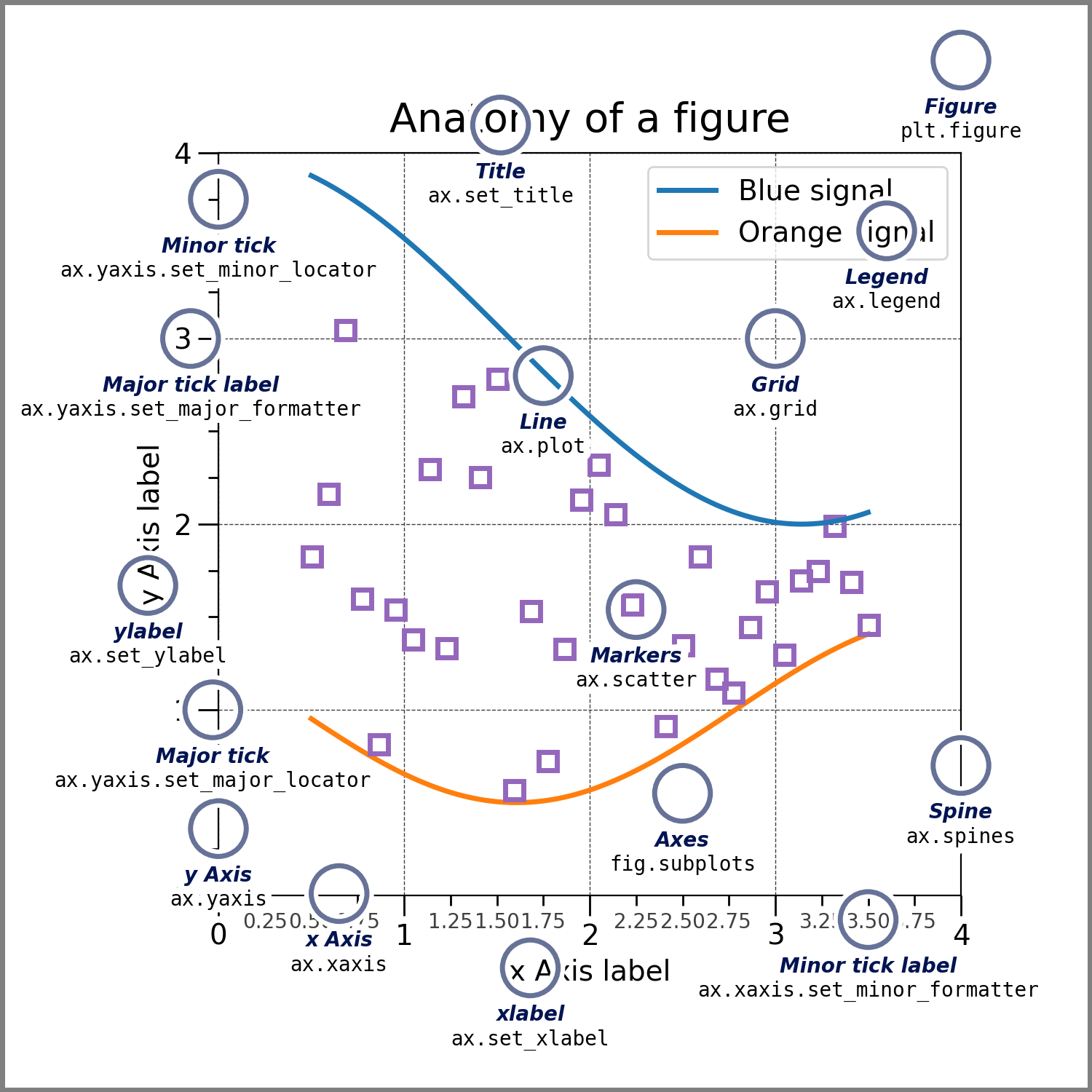
Now let us understand each part of a full-fledged figure in matplotlib. See the image below:

Matplotlib works best with only NumPy arrays. So if you have something else like a NumPy matrix or pandas dataframe, it is best to convert them to NumPy first. Pandas has a df.values attribute and NumPy has np.asarray(matrix) method to do this.
We only need to work with three types of objects in matplotlib. Try to understand these by seeing the picture below:

So we need to create a figure. Inside that figure, we create several axes. Inside those axes, there will be 2 or 3 axis (like real-life x-axis and y-axis). All of these are done below:
1x = np.linspace(0, 2, 100)
2
3fig, all_axes = plt.subplots(
4    2,3,              # The subplots will be in a grid of size 2x3
5    figsize=(20, 10), # The figure size is 20*80=1600 pixels width and 10*80=800 pixels height
6    dpi=80            # Define the density per pixel (number of pixels in 1 inch)
7)  # Create a figure and 6 axes
8
9((axs11, axs12, axs13),(axs21, axs22, axs23)) = all_axes
10
11axs11.plot(x, x**1, label='linear')       # Plot some data on the axes.
12axs12.plot(x, x**2, label='quadratic') # Plot more data on the axes...
13axs13.plot(x, x**3, label='cubic')     # ... and some more.
14
15axs21.plot(x, x**1, label='linear')     # ... and some more.
16axs22.plot(x, x**(1/2), label='quadratic')     # ... and some more.
17axs23.plot(x, x**(1/3), label='cubic')     # ... and some more.
18
19for axs in all_axes.reshape(-1):         # Loop through all axes. Here axes are np.array of shape (2,3). We reshape it to 1D.
20    axs.set_xlabel('x label')            # Add an x-label to the axes.
21    axs.set_ylabel('y label')            # Add a y-label to the axes.
22    axs.set_title("Simple Plot")         # Add a title to the axes.
23    axs.legend()                         # Add a legend.
24
25fig.show()
We will go through each type of plot one by one right after we introduce an interactive plot next.


